The first thing the user needs to do is to start the applet.
You could also download the source code from our web-site and compile it yourself. At this point in the tutorial we will assume that you can access the applet and that you have started it.
Once the applet has loaded, you will see the following screen:
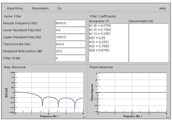
The applet can be split into three rows. The first row holds the Menu bar.

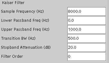
The second row has two columns. The first column is a Control panel where the parameters to design the filter or parameters to change the time scale of the plots are entered.
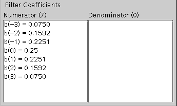
The second column in the second row is a Display panel that displays the filter coefficients after the filter is computed.
The third row consists of magnitude and phase plots of the filter computed.

The top section of the applet is the Menu bar. Using the menu bar, the user can choose a design algorithm, change the time scale in the plots, compute a filter, or reset the applet to its default settings.
To begin designing a filter, click on the "Algorithms" menu and choose an option. Once a filter design had been chosen, the parameters for the filter will be displayed on the Control Panel. Enter the parameters as shown in the Control panel. Then to compute the filter, click on the Compute option under the "Go" menu.
Other features that can be used in this applet are a tool to modify filter coefficients and the ability to zoom both the plots.
Filter Coefficients can be modified by choosing the Modify option under "Parameters" menu. This will display a panel in the Control panel that will look like as shown below.
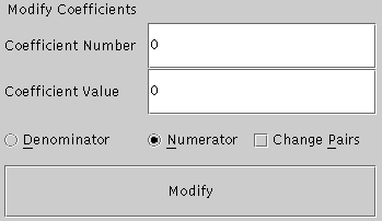
Enter the coefficient number and the value for that coefficient. Numerator or denominator coefficients can be changed by proper choice. The coefficients can also be changed in pairs using the Change Pairs option. After changing the coefficients, click on the Modify button in the bottom of the panel to update the value of the coefficients.
The time scales on the magnitude response plot can be changed choosing the Magnitude option under the "Parameters" menu. After this is done, the control panel will look like
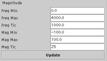
Enter the parameters as required on the text-fields and click on the "Update" button. There will be corresponding change in the Magnitude plot.
The phase plot also can be changed the same way as described for the magnitude plot except that the user needs to choose "Phase" option under "Parameters" menu.
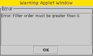
The applet has an extensive error messaging system. This will notify you if there is an error in the computation of a particular filter or if you have entered an invalid value for parameters. There error window looks like the following. By selecting OK, you will close the window and be able to correct the problem and try again.
When using the Butterworth filter algorithm, the main screen will look like as shown below
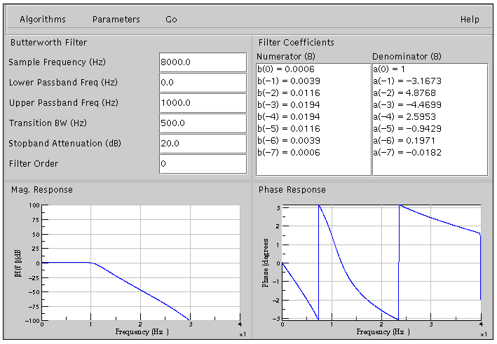
The control panel displays parameters like sample frequency (Hz), the lower passband frequency (Hz), upper passband frequency (Hz), transition bandwidth (Hz), stopband attenuation (dB), and the filter order. If the filter order is set to 0, the filter order used will be the optimal order as computed by the algorithm. The user can also set his own filter order by entering a non-negative, non-zero value in the filter order text-field.
Using the Chebyshev filter algorithm
When using the Chebyshev filter algorithm, the main screen will look like as shown below
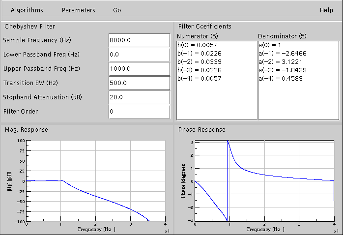
The control panel displays parameters like sample frequency (Hz), the lower passband frequency (Hz), upper passband frequency (Hz), transition bandwidth (Hz), stopband attenuation (dB), and the filter order. If the filter order is set to 0, the filter order used will be the optimal order as computed by the algorithm. The user can also set his own filter order by entering a non-negative, non-zero value in the filter order text-field. Note the ripples in the passband that did not exist in the Butterworth filter. Also, for the same specifications as that of Butterworth filter, Chebyshev filter gives a lower filter order.
Using the Bessel filter algorithm
When using the Bessel filter algorithm, the main screen will look like as shown below
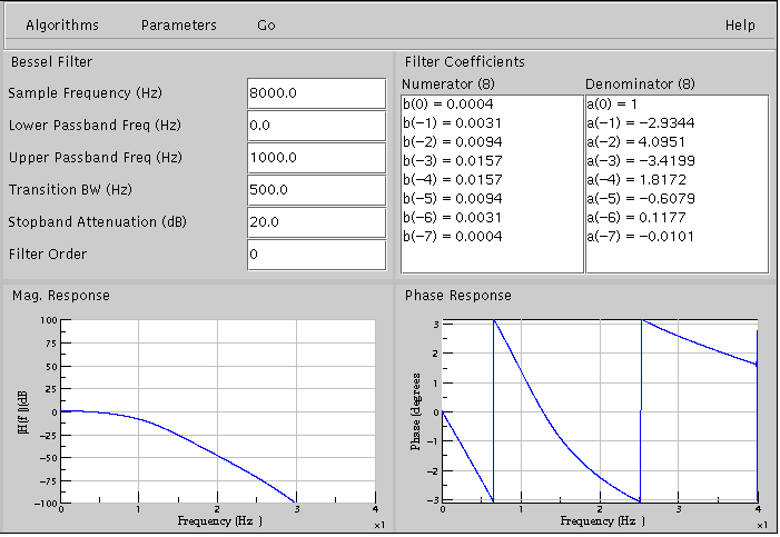
The control panel displays parameters like sample frequency (Hz), the lower passband frequency (Hz), upper passband frequency (Hz), transition bandwidth (Hz), stopband attenuation (dB), and the filter order. If the filter order is set to 0, the filter order used will be the optimal order as computed by the algorithm. The user can also set his own filter order by entering a non-negative, non-zero value in the filter order text-field. One important thing to note in the Bessel filter computation is that the filter order cannot exceed twenty five. If the user enters a filter order greater than twenty five, an error will be shown.
Using the Kaiser filter algorithm
When using the Kaiser filter algorithm, the main screen will look like the following.
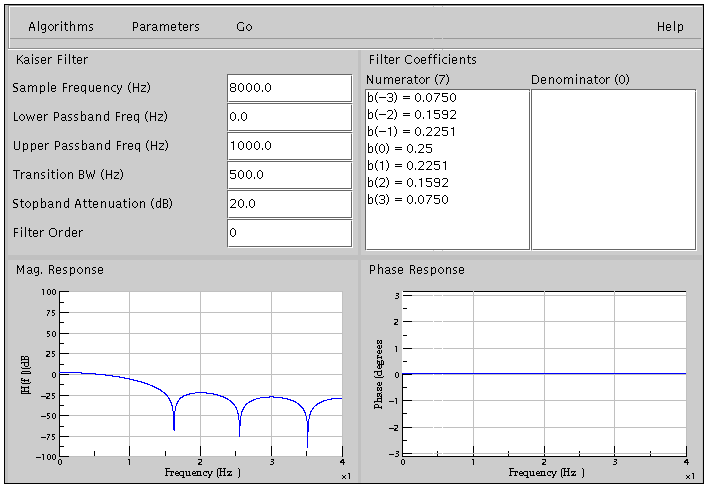
The user is able to select the sample frequency (Hz), the lower critical frequency (Hz), the upper critical frequency (Hz), the attenuation (dB), the transitional bandwidth (Hz), and the filter order. If the filter order is set to 0, the filter order used will be the optimal order as computed by the algorithm. Also, the filter odd needs to be odd else an error message will be shown.
When using the Parametric equalizer, the main screen will look like the following.
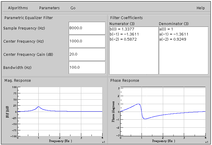
The user can set the Sample Frequency(Hz), Center Frequency(Hz), Gain at Center Frequency(dB) and Bandwidth(Hz). The parametric equalizer is a second order filter that can boost or cut a particular frequency by the given gain. If the gain value is positive, then that particular center frequency is boosted. If the gain value is negative, then the center frequency is attenuated by the value of gain. The sharpness of the boost or cut is controlled by the bandwidth.
If the gain is positive, then the parametric equalizer is a Resonator whose gain can be varied. If the gain is negative, then the parametric equalizer is a Notch filter.
When using an all-pass filter, the main screen will look as shown below.
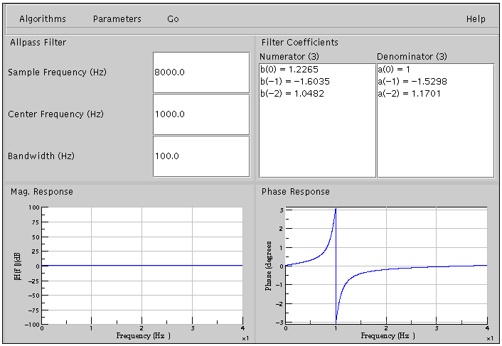
The user can set the Sample Frequency(Hz), Center Frequency(Hz) and Bandwidth(Hz). An all-pass filter is one which has constant magnitude response for all frequencies but the phase response varies based on the Sample Frequency(Hz), Center Frequency(Hz) and Bandwidth(Hz). While an all-pass filter can have any number of poles and zeros, the all-pass filter designed in this applet is a second order filter.
You can also define a filter by entering any coefficients you desire and compute the magnitude and phase. The main screen for this looks like the following.
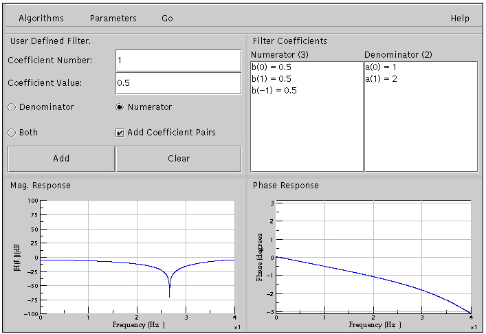
The screen above shows a filter having three numerator coefficients and two denominator coefficients. When entering filter coefficients, you can determine the coefficient number and value. You can also add coefficients to the numerator, denominator, or both simultaneously. It is also possible to add the coefficients in pairs. After entering each coefficient click on the 'Add' button to update the coefficient's list. Once you have entered all the desired coefficients, select the Compute option in the 'Go' menu.
